使用R语言进行时间序列分析

时间序列模型 $Y_t=m_t+s_t+X_t$ ，其中 $m_t$ 为趋势项， $s_t$ 为季节项（假设周期为 $d$ ，则 $s_t=s_{t+d}$ ）， $X_t$ 为平稳项（统计特性不随时间变化而改变）

一、对于趋势项的两种处理方式：

估计趋势并从原序列中去除，趋势的估计方法主要有以下几种：
- 滑动平均：
  
  可理解为Kernel Regression的一种特殊形式（Nadaraya–Watson estimator）
  
  假设滑动窗口为 $2h$ ，则趋势项 $\hat{m}_t=\frac{\sum_{i=1}^TI(\lvert{i-t}\rvert\leq{h})Y_i}{\sum_{i=1}^TI(\lvert{i-t}\rvert\leq{h})}$
- 线性回归：
  
  趋势项 $\hat{m}_t=\beta_0+\sum_{k=1}^p\beta_kt^k$ ， $p$ 通常取1或2
- Local Polynomial Regression：
  
  取离目标点最近的几个点进行加权线性回归
  
  假设窗口为 $2h$ ，核函数取为 $D(x)=\begin{cases}(1-\lvert{x}\rvert^3)^3, \text{if } \lvert{x}\rvert\leq{1} \\ 0, \text{otherwise}\end{cases}$ ，则需求解 $argmin_{\beta_k(t),k=0,1,...,p}\sum_{i=1}^TD(\frac{i-t}{h})[Y_i-\sum_{k=0}^p\beta_k(t)i^k]^2$
  
  趋势项 $\hat{m}_t=\beta_0(t)+\sum_{k=1}^p\beta_k(t)t^k$ ， $p$ 通常取1或2
- Splines Regression：
  - Truncated Polynomial
    
    假设选中的knots为 $t_1<t_2<...<t_K$ ，以cubic splines(i.e., degree=3)为例，它的基函数可取为 $B_1(t)=1,B_2(t)=t,B_3(t)=t^2,B_4(t)=t^3,B_5(t)=(t-t_1)^3_+,...,B_{K+4}(t)=(t-t_K)^3_+$
    
    趋势项 $\hat{m}_t=\sum_{j=1}^{K+4}\beta_jB_j(t)$
  - B-Spline
    
    和Truncated Polynomial等价但能有效减少计算量以及特征之间的共线性问题，仍以cubic splines(i.e., degree=3, M=degree+1=4)为例
    
    记 $t_0$ 和 $t_{K+1}$ 为boundary knots( $t_0<t_1, t_{K+1}>t_K$ )，令 $\tau_1=\tau_2=...=\tau_M=t_0, \tau_{K+M+1}=\tau_{K+M+2}=...=\tau_{K+2M}=t_{K+1}$ 以及 $\tau_{j+M}=t_j, j=1,2,...,K$
    
    记 $B_{i,m}(t)$ 为第i个阶数为m的基函数，有 $B_{i,1}(t)=\begin{cases}1, \text{if } \tau_i\leq{t}<\tau_{i+1} \\ 0, \text{otherwise}\end{cases}\text{ for }i=1,2,...,K+2M-1$ (注： $B_{i,1}(t)=0\text{ if }\tau_i=\tau_{i+1}$ )
    
    根据递推公式 $B_{i,m}(t)=\frac{t-\tau_i}{\tau_{i+m-1}-\tau_i}B_{i,m-1}(t)+\frac{\tau_{i+m}-t}{\tau_{i+m}-\tau_{i+1}}B_{i+1,m-1}(t)\text{ for }i=1,2,...,K+2M-m$ ，可以得到 $B_{i,4}(t)\text{ for }i=1,2,...,K+4$
    
    趋势项 $\hat{m}_t=\sum_{i=1}^{K+4}\beta_iB_{i,4}(t)$ （注：B-spline可以减少计算量的主要原因是生成的基函数 $B_{i,M}$ 最多仅在跨度为 $M+1$ 个knots范围内为非0值）
将相邻数据相减从而直接去除趋势，即 $\hat{Y}_t=Y_t-Y_{t-1}$

趋势估计应用（使用的数据集可从这里下载，提取码为16mm）

data = read.table("AvTempAtlanta.txt",header=T)
temp = as.vector(t(data[,-c(1,14)])) #去掉第一列和第十四列，转置并变为向量类型（R语言中的数组为列优先）
temp = ts(temp,start=1879,frequency=12)
ts.plot(temp,ylab="Temperature") #左图
## time
time.pts = c(1:length(temp)) #1,2,...,length(temp)
time.pts = c(time.pts - min(time.pts))/max(time.pts)
## Fit a moving average
mav.fit = ksmooth(time.pts, temp, kernel = "box")
temp.fit.mav = ts(mav.fit$y,start=1879,frequency=12)
## Fit a linear regression(quadraric polynomial)
x1 = time.pts
x2 = time.pts^2
lm.fit = lm(temp~x1+x2)
print(summary(lm.fit))
temp.fit.lm = ts(fitted(lm.fit),start=1879,frequency=12)
## Fit a local polynomial regression
loc.fit = loess(temp~time.pts)
temp.fit.loc = ts(fitted(loc.fit),start=1879,frequency=12)
## Fit a splines regression
library(mgcv)
gam.fit = gam(temp~s(time.pts))
temp.fit.gam = ts(fitted(gam.fit),start=1879,frequency=12)
## Compare all estimated trends
all.val = c(temp.fit.mav,temp.fit.lm,temp.fit.gam,temp.fit.loc)
ylim= c(min(all.val),max(all.val))
ts.plot(temp.fit.lm,lwd=2,col="green",ylim=ylim,ylab="Temperature") #右图
lines(temp.fit.mav,lwd=2,col="purple")
lines(temp.fit.gam,lwd=2,col="red")
lines(temp.fit.loc,lwd=2,col="brown")
legend(x=1900,y=64,legend=c("MAV","LM","GAM","LOESS"),lty = 1, col=c("purple","green","red","brown"))

二、对于季节项的两种处理方式：

估计季节项并从原序列中去除，估计方法主要有以下几种：
- 季节平均 $\hat{s}_k=average(Y_{k+jd}, j\geq0\text{ and }k+jd\leq{T}) \text{ for } k=1,2,...,d$
- 三角函数 $\hat{s}_t=\beta_0+\beta_1cos(2\pi{f}t)+\beta_2sin(2\pi{f}t)$ ， $f=1/d$
  - 若存在多个周期，则有 $\hat{s}_t=\beta_0+\sum_{j=1}^J[\beta_{1j}cos(2\pi{f}_jt)+\beta_{2j}sin(2\pi{f}_jt)]$
数据相减直接去除季节性，即 $\nabla_dY_t=Y_t-Y_{t-d}=m_t-m_{t-d}+X_t-X_{t-d}$

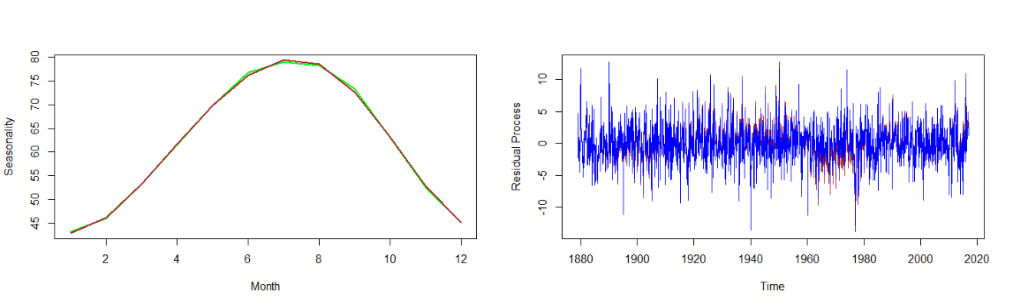
季节估计应用

library(TSA)
## Estimate seasonality using seasonal mean model
month = season(temp)
model1 = lm(temp~month-1) #all seasonal mean effects (model without intercept)
print(summary(model1))
## Estimate seasonality using cos-sin model
har2=harmonic(temp,2)
model2=lm(temp~har2)
print(summary(model2))
## Compare Seasonality Estimates
st1 = coef(model1)
st2 = fitted(model2)[1:12]
plot(1:12,st1,lwd=2,type="l",col='green',xlab="Month",ylab="Seasonality") #左图
lines(1:12,st2,lwd=2, col="brown")

趋势和季节估计应用

## Linear Regression
x1 = time.pts
x2 = time.pts^2
har2=harmonic(temp,2)
lm.fit = lm(temp~x1+x2+har2)
print(summary(lm.fit))
dif.fit.lm = ts((temp-fitted(lm.fit)),start=1879,frequency=12)
## Spline Regression for Trend and Linear Regression for Seasonality
gam.fit = gam(temp~s(time.pts)+har2)
print(summary(gam.fit))
dif.fit.gam = ts((temp-fitted(gam.fit)),start=1879,frequency=12)
## Compare approaches
ts.plot(dif.fit.lm,ylab="Residual Process",col="brown") #右图
lines(dif.fit.gam,col="blue")

三、平稳项

Auto-Covariance Function $cov(X_r,X_s)=E[(X_r-E[X_r])(X_s-E[X_s])]$

如果满足 $\begin{cases}E[X_t]=m\text{ for all t} \\ E[X_t^2]<\infty\text{ for all t} \\ cov(X_r,X_s)=cov(X_{r+t},X_{s+t})\text{ for all r,s,t}\end{cases}$ ，则序列 $\{X_t\}$ 是（弱）平稳序列

针对平稳序列，定义Auto-Covariance Function $\gamma_X(h)=cov(X_t, X_{t+h})$ , $t$ 可取任意值，则Auto-Correlation Function(ACF) $\rho_X(h)=\frac{\gamma_X(h)}{\gamma_X(0)}$

Sample Auto-Covariance Function $\hat{\gamma}_X(h)=\frac{1}{T}\sum_{t=1}^{T-h}(X_t-\bar{X})(X_{t+h}-\bar{X}),\text{ }0\leq{h}<T$ ，其中 $\bar{X}=\frac{1}{T}\sum_{t=1}^{T}X_t$

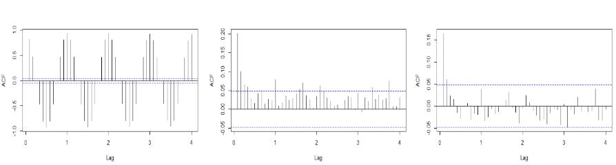
Sample ACF可表示为 $\hat{\rho}_X(h)=\frac{\hat{\gamma}_X(h)}{\hat{\gamma}_X(0)}$

acf(temp,lag.max=12*4,main="") #左图（用于对比）
acf(dif.fit.lm,lag.max=12*4,main="") #中图
acf(dif.fit.gam,lag.max=12*4,main="") #右图

四、完整案例应用

使用的数据集可从这里下载，提取码为uqq8

Process Data

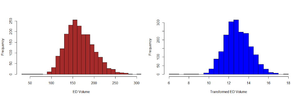
edvoldata = read.csv("EGDailyVolume.csv",header=T)
## Process Dates
year = edvoldata$Year
month = edvoldata$Month
day = edvoldata$Day
datemat = cbind(as.character(day),as.character(month),as.character(year))
paste.dates = function(date){
     day = date[1]; month=date[2]; year = date[3]
     return(paste(day,month,year,sep="/"))
 }
dates = apply(datemat,1,paste.dates)
dates = as.Date(dates, format="%d/%m/%Y")
edvoldata = cbind(dates,edvoldata)
## Transform ED Volume data(Stabilize Variance)
Volume.tr = sqrt(edvoldata$Volume+3/8)
hist(edvoldata$Volume,nclass=20,xlab="ED Volume", main="",col="brown") #左图
hist(Volume.tr,nclass=20,xlab= "Transformed ED Volume", main="",col="blue") #右图

Trend and Seasonality

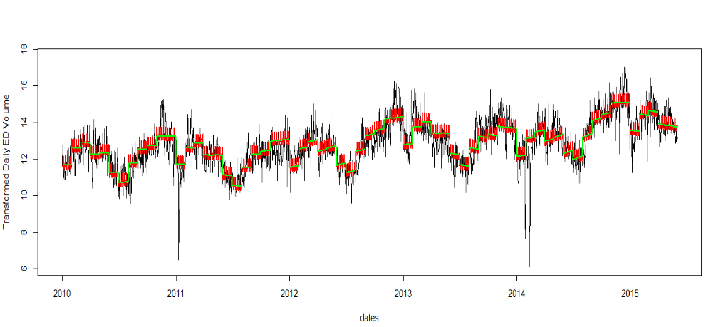
library(mgcv)
time.pts = c(1:length(Volume.tr))
time.pts = c(time.pts - min(time.pts))/max(time.pts)
## Model Trend + Monthly Seasonality
## Use Splines Trend and Seasonal Mean Model
month = as.factor(format(dates,"%b"))
gam.fit.seastr.1 = gam(Volume.tr~s(time.pts)+month)
print(summary(gam.fit.seastr.1))
vol.fit.gam.seastr.1 = fitted(gam.fit.seastr.1)
## Add day-of-the-week seasonality
week = as.factor(weekdays(dates))
gam.fit.seastr.2 = gam(Volume.tr~s(time.pts)+month+week)
print(summary(gam.fit.seastr.2))
vol.fit.gam.seastr.2 = fitted(gam.fit.seastr.2)
## Compare the two fits: with & without day-of-the-week seasonality
plot(dates,Volume.tr,type="l",ylab="Transformed Daily ED Volume") #下图
lines(dates,vol.fit.gam.seastr.2,lwd=2,col="red")
lines(dates,vol.fit.gam.seastr.1,lwd=2,col="green")

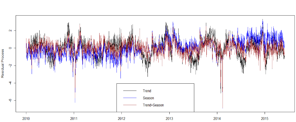
Stationary Residual

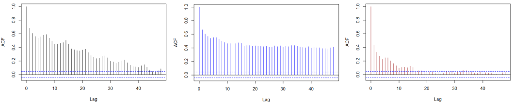
## Residual Process: Trend Removal
gam.fit = gam(Volume.tr~s(time.pts))
vol.fit.gam = fitted(gam.fit)
resid.1 = Volume.tr-vol.fit.gam
## Residual Process: Seasonal Removal
lm.fit.seastr.2 = lm(Volume.tr~month+week)
vol.fit.lm.seastr.2 = fitted(lm.fit.seastr.2)
resid.2 = Volume.tr-vol.fit.lm.seastr.2
## Residual Process: Trend & Seasonal Removal
resid.3 = Volume.tr-vol.fit.gam.seastr.2
## Compare Residuals
y.min = min(c(resid.1,resid.2,resid.3))
y.max = max(c(resid.1,resid.2,resid.3))
plot(dates, resid.1, ylim=c(y.min, y.max), type="l", ylab="Residual Process") #上图  
lines(dates,resid.2,col="blue")
lines(dates,resid.3,col="brown")
legend("bottom",legend=c("Trend","Season","Trend+Season"),lty = 1, col=c("black","blue","brown")) 
## ACF
acf(resid.1,lag.max=12*4,main="") #左下图
acf(resid.2,lag.max=12*4,main="",col="blue") #中下图
acf(resid.3,lag.max=12*4,main="",col="brown") #右下图